In the second part of this three part series, I discussed the fluid flow analysis software and the three step process that we use to build models. In the third and final part, I’ll go through an actual ventilation system design project that we modeled in the FFA software.
Example Project
The ventilation system that we will are using as our example was for a pipeline compressor station. The system was designed to have a powered supply and a gravity exhaust. The basic requirements of the system were:
- Positive pressure with air flow at 20,200 CFM;
- Hoods with guards/bird screens;
- Silencing treatment to reduce noise to 50 dBA at 50 feet; and
- Backdraft dampers.
The two drawings below show how the system was designed to meet these requirements:
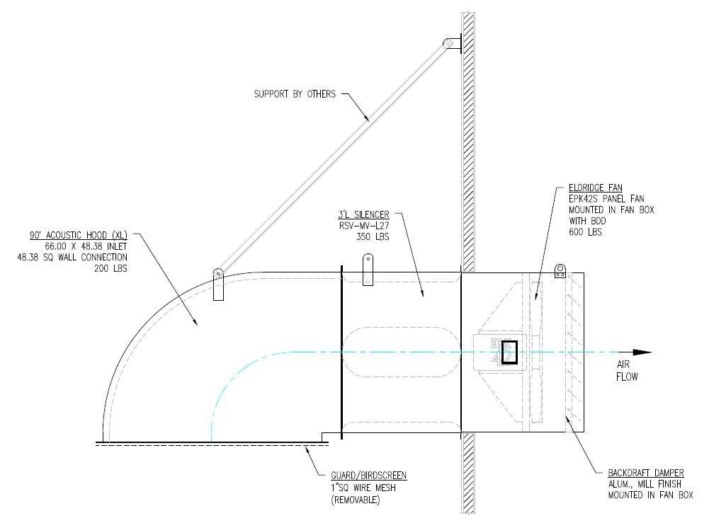
POWERED SUPPLY
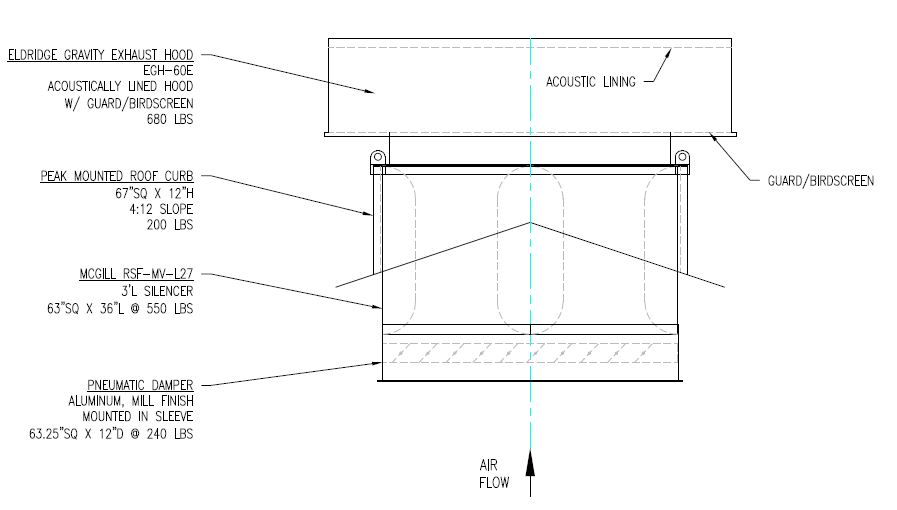
GRAVITY EXHUAST
Model Building
Following the steps in our model building process that we covered in part 2, we will start with identifying the separate components of the ventilation system:
- Supply Hood Guard/Bird Screen
- Supply Hood Intake Opening
- Supply Hood 90 deg. Turn
- Supply Silencer
- Supply Backdraft Damper
- Inside Building Geometry
- Inside Building Geometry
- Exhaust Damper
- Exhaust Silencer
- Exhaust Hood 180 deg. Turn
- Exhaust Hood Exit Opening
I want to point out a few things we learned about separating the components for modeling purposes. All openings in a ventilation system will have entrance or exit pressure losses. However, when an opening is the intake or exhaust of a piece of equipment such as a damper, you will need to determine if the manufacture’s pressure loss coefficients for the equipment include the entrance or exit loss. In the case of the Supply and Exhaust Dampers in our example system, the manufactures did include the entrance/exit pressure losses in their coefficients so we didn’t need to model these openings separately.
When modeling a ventilation system for a building, the building itself becomes a component as if it were a piece of duct work connecting the supply and exhaust components. Unless there is some significant obstacles between the supply and exhaust, the assumption should be that there is no pressure drop associated with the building component.
After we determined which were the separate components of the ventilation system, we calculated the loss coefficient for each component. For the equipment such as dampers and silencers, we used the manufacturer’s coefficients. However, because the supply and exhaust hoods were our unique designs for this project, we used data in the Handbook of Hydraulic Resistance by I.E. Idel’chik to calculate their loss coefficients.
Modeling Results
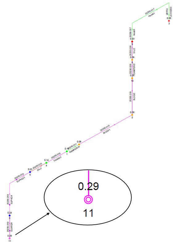
With the component data entered into the model as well as the required air flow of 20,200 CFM, the software was able to show us what that the total static pressure for the system is 0.29” wg. Below is the output from the software with total static pressure shown at the guard/bird screen for the supply hood.
The next step was to input the fan curve of the fan that we choose for the system. The output from the software with the fan included in the model is shown below.
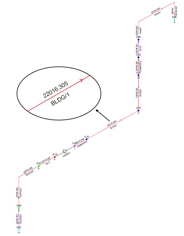
What the software showed us was that the actual flow in the system would be 22,016 CFM. The only way that the software was able to do that was because we gave it a fan curve and not a single data point. Because the air flow is more than what was required by the system specification, we will provide slightly more flow to the customer’s application than it requires, thus exceeding our customer’s expectations.
Conclusion
We hope that you have enjoyed our blog series on Using Flow Analysis. It is a very useful tool when a ventilation system is very complex. However, as the example above showed, it is also a good way to check assumptions and hand calculations for very simple systems when there are very precise requirements for the application.